Investing in Performance: Fine-tune small models with LLM insights - a CFM case study
Overview: This article presents a deep dive into Capital Fund Management’s (CFM) use of open-source large language models (LLMs) and the Hugging Face (HF) ecosystem to optimize Named Entity Recognition (NER) for financial data. By leveraging LLM-assisted labeling with HF Inference Endpoints and refining data with Argilla, the team improved accuracy by up to 6.4% and reduced operational costs, achieving solutions up to 80x cheaper than large LLMs alone.
In this post, you will learn:
- How to use LLMs for efficient data labeling
- Steps for fine-tuning compact models with LLM insights
- Deployment of models on Hugging Face Inference Endpoints for scalable NER applications
This structured approach combines accuracy and cost-effectiveness, making it ideal for real-world financial applications.
| Model | F1-Score (Zero-Shot) | F1-Score (Fine-Tuned) | Inference Cost (per hour) | Cost Efficiency |
|---|---|---|---|---|
| GLiNER | 87.0% | 93.4% | $0.50 (GPU) / $0.10 (CPU) | Up to 80x cheaper |
| SpanMarker | 47.0% | 90.1% | $0.50 (GPU) / $0.10 (CPU) | Up to 80x cheaper |
| Llama 3.1-8b | 88.0% | N/A | $4.00 | Moderate |
| Llama 3.1-70b | 95.0% | N/A | $8.00 | High Cost |
Capital Fund Management (CFM) is an alternative investment management firm headquartered in Paris, also has teams in New York City and London currently overseeing assets totaling 15.5 billion dollars.
Employing a scientific approach to finance, CFM leverages quantitative and systematic methods to devise superior investment strategies.
CFM has been working with Hugging Face's Expert Support to stay updated on the latest advancements in machine learning and harness the power of open-source technology for their wide range of financial applications. One of the collaboration's main goals has been to explore how CFM can benefit from efficiently using open-source Large Language Models (LLMs) to enhance their existing machine learning use cases. Quantitative hedge funds rely on massive amounts of data to inform decisions about whether to buy or sell specific financial products. In addition to standard data sources from financial markets (e.g., prices), hedge funds are increasingly extracting insights from alternative data, such as textual information from news articles. One major challenge in incorporating news into fully automated trading strategies is accurately identifying the products or entities (e.g., companies, stocks, currencies) mentioned in the articles. While CFM’s data providers supply these tags, they can be incomplete and require further validation.
CFM explored several approaches to improve financial entity recognition, including zero-shot NER using LLMs and smaller models, LLM-assisted data labeling with Hugging Face Inference Endpoints and Argilla, and fine-tuning smaller models on curated datasets. These approaches not only leverage the versatility of large models but also address the challenges of cost and scalability in real-world financial applications.
Among open-source models, the Llama 3.1 series by Meta stood out due to its strong performance across benchmarks, making it a top choice for generating synthetic annotations. These LLMs were pivotal in creating high-quality labeled datasets, combining automation and human expertise to streamline the labeling process and enhance model performance in financial NER tasks.
Table of Content
- NER on the Financial News and Stock Price Integration Dataset
- LLM-Assisted data labeling with Llama
- Performance of zero-shot approaches for financial NER
- Improving performance of compact models with fine-tuning on LLM-assisted labeled dataset
- Weak Supervision vs. LLM-assisted labeling
NER on the Financial News and Stock Price Integration Dataset
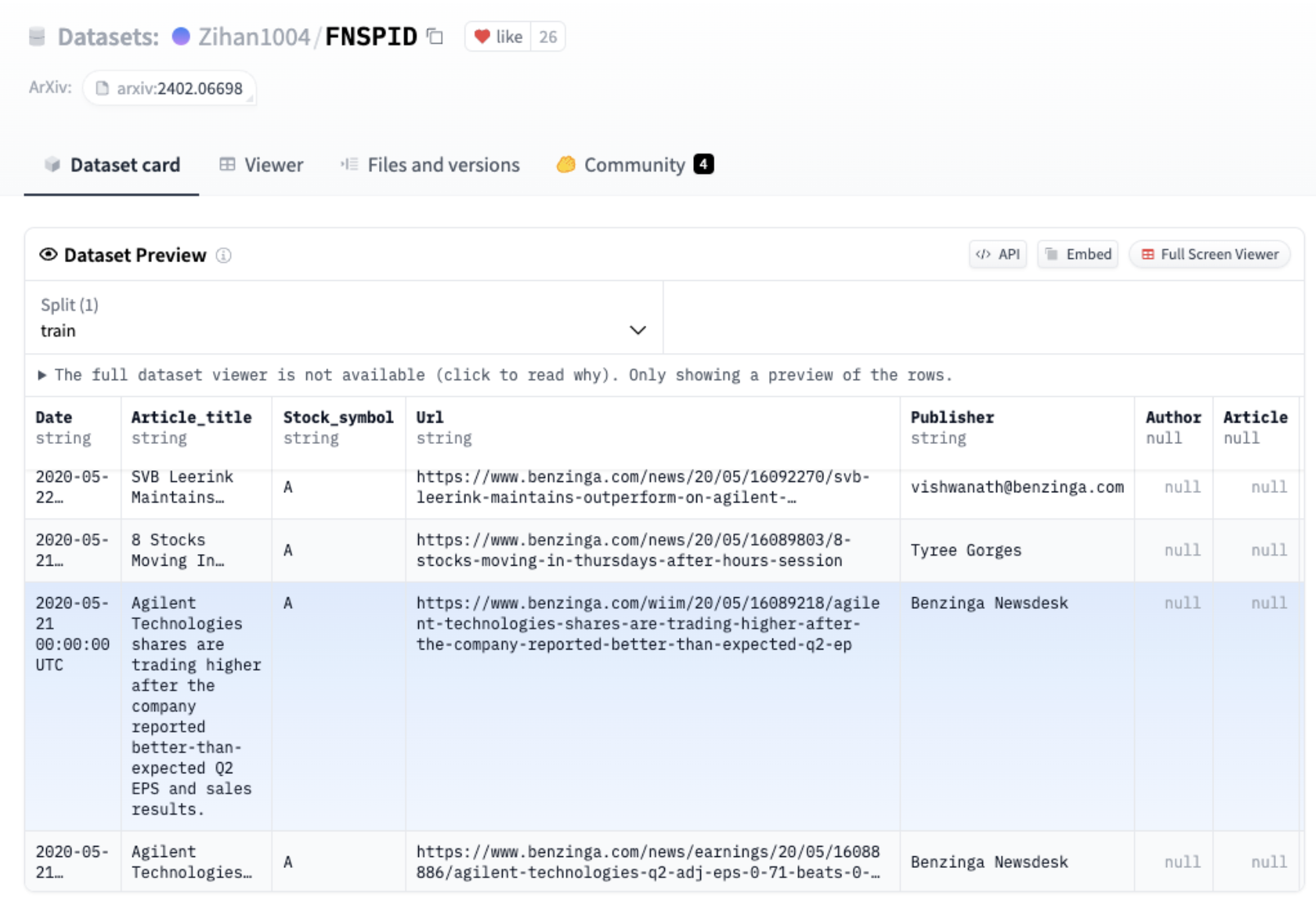
Our focus on this use case was to extract company names from news headlines from the Financial News and Stock Price Integration Dataset (FNSPID). It is composed of news headlines and articles associated with corresponding stock symbols coming from several sources such as Bloomberg, Reuters, Benzinga and others. After analyzing the various news sources, we found that news from Benzinga had no missing stock symbol values. This subset of the dataset contains ~900k samples. As a result, we decided to reduce our dataset to Benzinga headlines for a more consistent and reliable analysis.
Dataset preview of FNSPID
    {"example 1": "Black Diamond Stock Falling After Tweet"} -> Black Diamond
    {"example 2": "Dun & Bradstreet Acquires Avention For $150M"} ->  Dun & Bradstreet, Avention
    {"example 3": "Fast Money Picks For April 27"} -> No company
Example samples and target predictions for the task
LLM-Assisted data labeling with Llama
To effectively compare different approaches, we first need to consolidate a reliable dataset that will serve as a foundation for evaluating the candidate methods. This dataset will be used for both testing the performance of models in zero-shot settings and as a base for fine-tuning.
We used Llama-assisted data labeling to streamline and enhance the annotation process by having Llama 3.1 generate labels for dataset samples. These auto-generated labels were then manually reviewed using the open-source data annotation platform Argilla. This approach allowed us to speed up the labeling process while ensuring the quality of the annotations.
Deploy Llama3.1-70b-Instruct with Hugging Face Inference Endpoints
To securely and quickly get access to a Llama3.1-70-Instruct deployment we opted for Hugging Face Inference Endpoints.
Hugging Face Inference Endpoints provide a straightforward and secure solution for deploying machine learning models in production environments. They enable developers and data scientists to build AI applications without the need to manage infrastructure, simplifying deployment to just a few clicks.
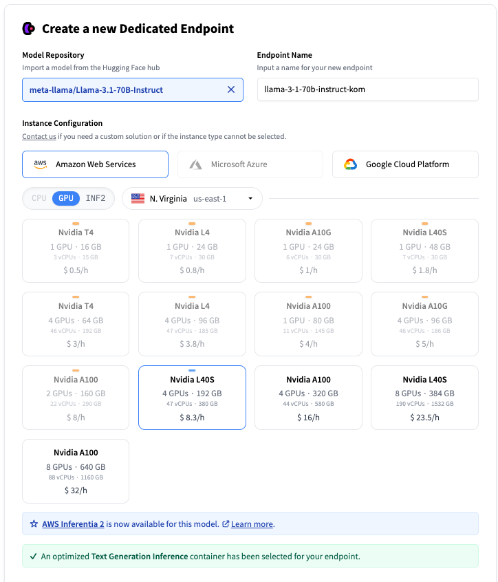
To access Inference Endpoints we logged in as a member of the CapitalFundManagement organization on the Hugging Face Hub, then accessed the service at https://ui.endpoints.huggingface.co . To start a new deployment we create on New then select meta-llama/Llama-3.1-70B-Instruct
Endpoint creation on the Inference Endpoints UI
You can select on which cloud provider the hardware will be hosted, the region, and the type of instance. Inference Endpoints suggest an instance type based on the model size, which should be big enough to run the model. Here an instance with 4 Nvidia L40S is selected. When LLM is selected, an automated container is selected running Text Generation Inference for optimized inference.
When clicking on the “Create Endpoint” the deployment is created and the endpoint will be ready in a few minutes. To get more information about Inference Endpoints setup, visit https://huggingface.co/docs/inference-endpoints.
Endpoint running on the Inference Endpoints UI
Once our endpoint is running, we will use the endpoint URL provided to send requests to it.
Prompting Llama for NER
Before sending requests, we needed to design a prompt that would guide the model effectively to generate the desired output. After several rounds of testing, we structured the prompt into multiple sections to address the task accurately:
Role Definition: The model is positioned as a financial expert with strong English skills.
Task Instructions: The model is instructed to extract company names linked to stocks mentioned in headlines, while excluding stock indices often found in titles.
Expected Output: The model must return a dictionary with:
"result": Exact company names or stock symbols."normalized_result": Standardized company names corresponding to those in"result".
Few-shot Examples: A series of input-output examples to demonstrate the expected behavior and ensure consistency in performance across varied inputs. These examples help the model understand how to distinguish relevant entities and format its output correctly. Each example illustrates different headline structures to prepare the model for a range of real-world cases.
SYSTEM_PROMPT = “””
###Instructions:###
You are a financial expert with excellent English skills.
Extract only the company names from the following headlines that are related to a stock discussed in the article linked to the headline.
Do not include stock indices such as "CAC40" or "Dow Jones".

##Expected Output:##
Return a dictionary with:
A key "result" containing a list of company names or stock symbols. Make sure to return them exactly as they are written in the text even if the original text has grammatical errors. If no companies or stocks are mentioned, return an empty list.
A key "normalized_result" containing the normalized company names corresponding to the entries in the "result" list, in the same order. This list should have the same size as the "result" list.

##Formatting:##
Do not return companies not mentioned in the text.

##Example Outputs##

Input: "There's A New Trading Tool That Allows Traders To Trade Cannabis With Leverage"
Output: {"result": [], "normalized_result": []}
Input: "We explain AAPL, TSLA, and MSFT report earnings"
Output: {"result": ["AAPL", "TSLA", "MSFT"], "normalized_result": ["Apple", "Tesla", "Microsoft"]}
Input: "10 Biggest Price Target Changes For Friday"
Output: {"result": [], "normalized_result": []}
Input: "'M' is For Microsoft, and Meh"
Output: {"result": ["Microsoft"], "normalized_result": ["Microsoft"]}
Input: "Black Diamond: The New North Face? (BDE, VFC, JAH, AGPDY.PK)"
Output: {"result": ['Black Diamond', 'North Face', 'BDE', 'VFC','JAH','AGPDY.PK'], "normalized_result": ['Black Diamond','The North Face', 'BPER Banca', 'VF Corporation','Jarden Corporation','AGP Diagnostics']}
“””
Get predictions from the endpoint
Now that we have our prompt and endpoint ready, the next step is to send requests using the titles from our dataset. To do this efficiently, we'll use the AsyncInferenceClient from the huggingface_hub library. This is an asynchronous version of the InferenceClient, built on asyncio and aiohttp. It allows us to send multiple concurrent requests to the endpoint, making the processing of the dataset faster and more efficient.
from huggingface_hub import AsyncInferenceClient

# Initialize the Hugging Face AsyncInferenceClient
client = AsyncInferenceClient(base_url="https://your-endpoint-url.huggingface.cloud")
To make sure the model replies a structured output, we will use guidance with a specific Pydantic schema Companies
from pydantic import BaseModel
from typing import List, Dict, Any

# This class defines the expected structure for the output using Pydantic.
class Companies(BaseModel):
    """
    Pydantic model representing the expected LLM output.

    Attributes:
        result (List[str]): A list of company names or results from the LLM.
        normalized_result (List[str]): A list of 'normalized' company names, i.e., processed/cleaned names.
    """
    result: List[str]
    normalized_result: List[str]

grammar: Dict[str, Any] = {
    "type": "json_object",
    "value": Companies.schema()
    # This instructs the LLM to return a JSON with "result" and "normalized_result" as keys
}
We also set generation parameters:
max_tokens: int = 512  # Maximum number of tokens to generate in the response
temperature: float = 0.1  # Controls randomness in the output (lower values are more deterministic)
Now we define our functions to send requests to the endpoint and parse output:
async def llm_engine(messages: List[Dict[str, str]]) -> str:
    """
    Function to send a request to the LLM endpoint and get a response.

    Args:
        messages (List[Dict[str, str]]): A list of messages to pass to the LLM.

    Returns:
        str: The content of the response message or 'failed' in case of an error.
    """
    try:
        # Send the request to the LLM endpoint asynchronously
        response = await client.chat_completion(
            messages=messages,
            model="ENDPOINT",  # Replace with your model endpoint
            temperature=temperature,
            response_format=grammar,
            max_tokens=max_tokens
        )
        # Extract the content of the response message
        answer: str = response.choices[0].message.content
        return answer
    except Exception as e:
        # Handle any exceptions that occur during the request
        print(f"Error in LLM engine: {e}")
        return "failed"

def parse_llm_output(output_str: str) -> Dict[str, Any]:
    """
    Parse the JSON-like output string from an LLM into a dictionary.

    Args:
        output_str (str): The string output from an LLM, expected to be in JSON format.

    Returns:
        Dict[str, Any]: A dictionary parsed from the input JSON string with a 'valid' flag.
    """
    try:
        # Parse the JSON string into a dictionary
        result_dict: Dict[str, Any] = json.loads(output_str)
        result_dict["valid"] = True
        return result_dict
    except json.JSONDecodeError as e:
        # Handle JSON parsing errors and return a default structure
        print(f"Error decoding JSON: {e}")
        return {
            "result": [output_str],
            "normalized_result": [output_str],
            "valid": False
        }
We test the endpoint with a single example:
messages = [
           {"role": "system", "content": SYSTEM_PROMPT},
            {"role": "user", "content": "Some stocks i like buying are AAPL, GOOG, AMZN, META"}
            ]
response = await llm_engine(messages)
print(parse_llm_output(response))
{"normalized_result": ["Apple", "Alphabet", "Amazon", "Meta Platforms"], "result": ["AAPL", "GOOG", "AMZN", "META"]}
Now, we create a process_batch function to handle sending requests in manageable batches, preventing the API endpoint from becoming overwhelmed or hitting rate limits. This batching approach allows us to efficiently process multiple requests concurrently without saturating the server, reducing the risk of timeouts, rejected requests, or throttling. By controlling the flow of requests, we ensure stable performance, faster response times, and easier error handling while maximizing throughput.
import asyncio

async def process_batch(batch):
    """
    Get the model output for a batch of samples.

    This function processes a batch of samples by sending them to the LLM and
    gathering the results concurrently.

    Args:
        batch (List[Dict[str, str]]): A list of dictionaries where each dictionary
                                      contains the data for a single sample, including
                                      an "Article_title".

    Returns:
        List[str]: A list of responses from the LLM for each sample in the batch.
    """

    list_messages = []

    # Loop through each sample in the batch
    for sample in batch:
        messages = [
           {"role": "system", "content": SYSTEM_PROMPT},
           {"role": "user", "content": sample["Article_title"]}
        ]
        list_messages.append(messages)

    # Use asyncio.gather to send requests to the LLM concurrently for all message sequences
    return await asyncio.gather(*[llm_engine(messages) for messages in list_messages])
We will run inference over the dataset:
from datasets import load_dataset, Dataset

#Streaming data from Huggingface Hub to avoid downloading the entire dataset
dataset = load_dataset("Zihan1004/FNSPID", streaming=True)

iterable_dataset = iter(dataset["train"])

# Create a batch of samples from remote dataset
def get_sample_batch(iterable_dataset, batch_size):
    batch = []
    try:
        for _ in range(batch_size):
            batch.append(next(iterable_dataset))
    except StopIteration:
        pass
    return batch
And we create the main inference loop:
#Main loop
batch_size = 128
i= 0
len_extracted = 0

while True:
    batch = get_sample_batch(iterable_dataset, batch_size)
    #batch = samples[i * batch_size : (i+1) * batch_size]
    predictions = await process_batch(batch)
    parsed_predictions = [parse_llm_output(_pred) for _pred in predictions]
    try :
        parsed_dataset = [
            {"Article_title": sample["Article_title"],
             "predicted_companies": pred["result"],
             "normalized_companies":pred.get("normalized_result", ""),
             "valid": pred["valid"]} for sample, pred in zip(batch, parsed_predictions)
            ]
    except Exception as e :
        print(i,e)
        continue

    # Write parsed_dataset to a JSON file
    with open(os.path.join(CHECKPOINT_DATA, f"parsed_dataset_{i}.json"), 'w') as json_file:
        json.dump(parsed_dataset, json_file, indent=4)  # Use json.dump to write data to a JSON file

    len_extracted += len(parsed_dataset)
    i+= 1
    print(f"Extracted: {len_extracted} samples")
    if len(batch) < batch_size:
        break
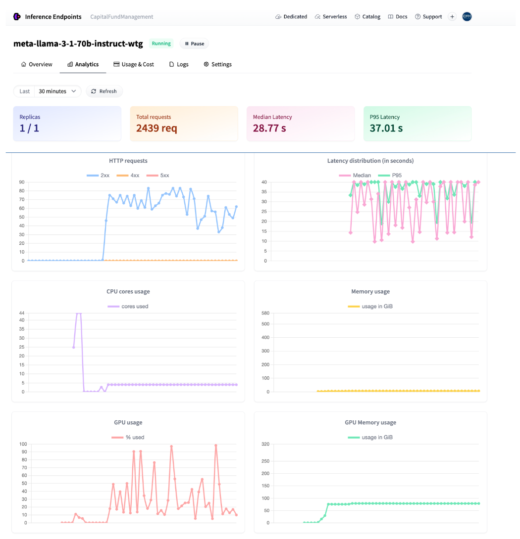
When the inference is running we can monitor the traffic directly from the UI
Endpoint analytics
It took about 8 hours to process the whole dataset with 900k samples which costs ~$70.
Review predictions with Argilla
With the labeled data generated from our LLM, the next step is to curate a high-quality subset to ensure reliable evaluation of different methods, including zero-shot and fine-tuning approaches. This carefully reviewed dataset will also serve as a foundational base for fine-tuning smaller models. The entire labeled dataset by the LLM can be also used for fine-tuning in a weak supervision framework.
Dataset sampling and splitting
To create a manageable sample size for review, we used LLM labels and clustered company names using fuzzy matching with the rapidfuzz library. We applied the cdist function to compute Levenshtein distances between companies and clustered them with a threshold of 85. A representative company was selected for each cluster, and Llama predictions were mapped accordingly. Finally, we sampled 5% of news headlines from each company-related cluster and 5% from headlines without any companies resulting in a dataset of 2714 samples.
Then using metadata, the sampled dataset is divided into three parts:
Train: News from 2010 to 2016, used for training small ML models - 2405 samples
Validation: News from 2017 to 2018, for hyperparameters tuning - 204 samples
Test: News from 2019 to 2020, used to evaluate the model on unseen data. - 105 samples
Once created, we set up an annotation tool, Argilla, to ease the annotation process.
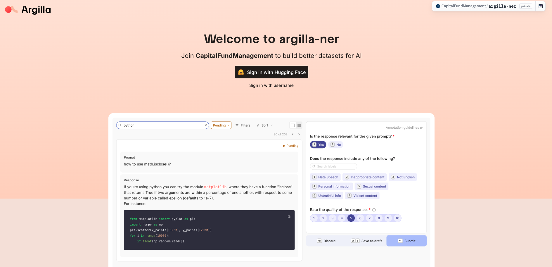
Argilla is an open-source tool, integrated into the Hugging Face ecosystem that excels at gathering human feedback for a wide range of AI projects. Whether you're working on traditional NLP tasks like text classification and NER, fine-tuning large language models (LLMs) for retrieval-augmented generation (RAG) or preference tuning, or developing multimodal models like text-to-image systems, Argilla provides the tools needed to collect and refine feedback efficiently. This ensures your models continuously improve based on high-quality, human-validated data.
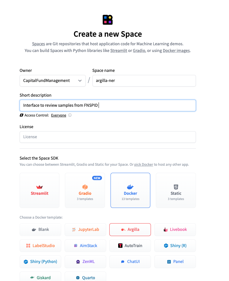
An Argilla interface can be set up directly through Hugging Face Spaces and this is what we opted for. Check out the documentation to start your own interface and go to https://huggingface.co/new-space .
Create Argilla Space on the Hub
Argilla homepage on Spaces
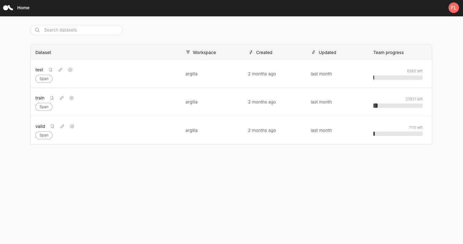
Argilla datasets view
Once the interface is created, we can connect programmatically to it using the Argilla python SDK. To get ready to annotate we followed the following steps:
- We connect to our interface using credentials provided in the settings.
import argilla as rg
client = rg.Argilla(
    api_url="https://capitalfundmanagement-argilla-ner.hf.space",
    api_key="xxx",
    headers={"Authorization": f"Bearer {HF_TOKEN}"},
    verify = False)
- We create the guidelines for the annotation, and generate the task specific dataset. Here, we specify the SpanQuestion task. We then generate a train, a validation and test dataset objects with the defined settings.
import argilla as rg  # Import the Argilla library.


# Define the label for token classification (e.g., "Company").
labels = ["Company"]


# Define settings for the annotation task.
settings = rg.Settings(
    guidelines="Classify individual tokens according to the specified categories, ensuring that any overlapping or nested entities are accurately captured.",
    fields=[rg.TextField(name="text", title="Text", use_markdown=False)],
    questions=[rg.SpanQuestion(
        name="span_label",
        field="text",
        labels=labels,
        title="Classify the tokens according to the specified categories.",
        allow_overlapping=False,
    )],
)


# Create datasets with the same settings for training, validation, and testing.
train_dataset = rg.Dataset(name="train", settings=settings)
train_dataset.create()

valid_dataset = rg.Dataset(name="valid", settings=settings)
valid_dataset.create()

test_dataset = rg.Dataset(name="test", settings=settings)
test_dataset.create()
- We populate the dataset with news headlines from the different datasets
train_records = [rg.Record(fields={"text": title}) for title in train_df["Article_title"]]
valid_records = [rg.Record(fields={"text": title}) for title in valid_df["Article_title"]]
test_records = [rg.Record(fields={"text": title}) for title in test_df["Article_title"]]

train_records_list = [{"id": record.id, "text": record.fields["text"]} for record in train_records]
valid_records_list = [{"id": record.id, "text": record.fields["text"]} for record in valid_records]
test_records_list = [{"id": record.id, "text": record.fields["text"]} for record in test_records]

train_dataset.records.log(train_records)
valid_dataset.records.log(valid_records)
test_dataset.records.log(test_records)
- In this step, we incorporate predictions from various models. Specifically, we add Llama 3.1 predictions into Argilla, where each entity is represented as a dictionary containing a start index, end index, and a label (in this case, 'Company')."
train_data = [{"span_label": entity,"id": id,} for id, entity in zip(train_ids, train_entities_final)]
valid_data = [{"span_label": entity,"id": id,} for id, entity in zip(valid_ids, valid_entities_final)]
test_data = [{"span_label": entity,"id": id,} for id, entity in zip(test_ids, test_entities_final)]

train_dataset.records.log(records=train_data, batch_size = 1024)
valid_dataset.records.log(records=valid_data, batch_size = 1024)
test_dataset.records.log(records=test_data, batch_size = 1024)
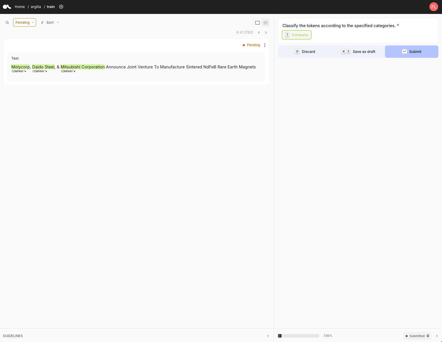
Argilla annotation view
The annotation interface displays the text to be annotated, along with its status (either pending or submitted). Annotation guidelines are presented on the right side of the screen. In this case, we have one label, 'Company.' To annotate, we first select the label, then highlight the relevant text in the sentence. Once all entities are selected, we click 'submit' to finalize the annotation.
Duration of annotation
Using pre-computed Llama labels significantly accelerates the annotation process, reducing the time per sample to just 5 to 10 seconds, compared to roughly 30 seconds for raw, unprocessed samples. This efficiency leads to a substantial time saving, allowing us to complete the annotation of 2,714 samples in around 8 hours. The efficiency gains are even more pronounced for more complex tasks than NER, where the time saved with pre-computed labels or generation becomes significantly greater.
Performance of zero-shot approaches for financial NER
With a high-quality, reviewed dataset in place, we can now experiment with different approaches for zero-shot NER. We tested four models:
Small Language Models:
- GLINER
- SpanMarker Large Language Models (LLMs):
- Llama-3.1-8b
- Llama-3.1-70b
- GLiNER
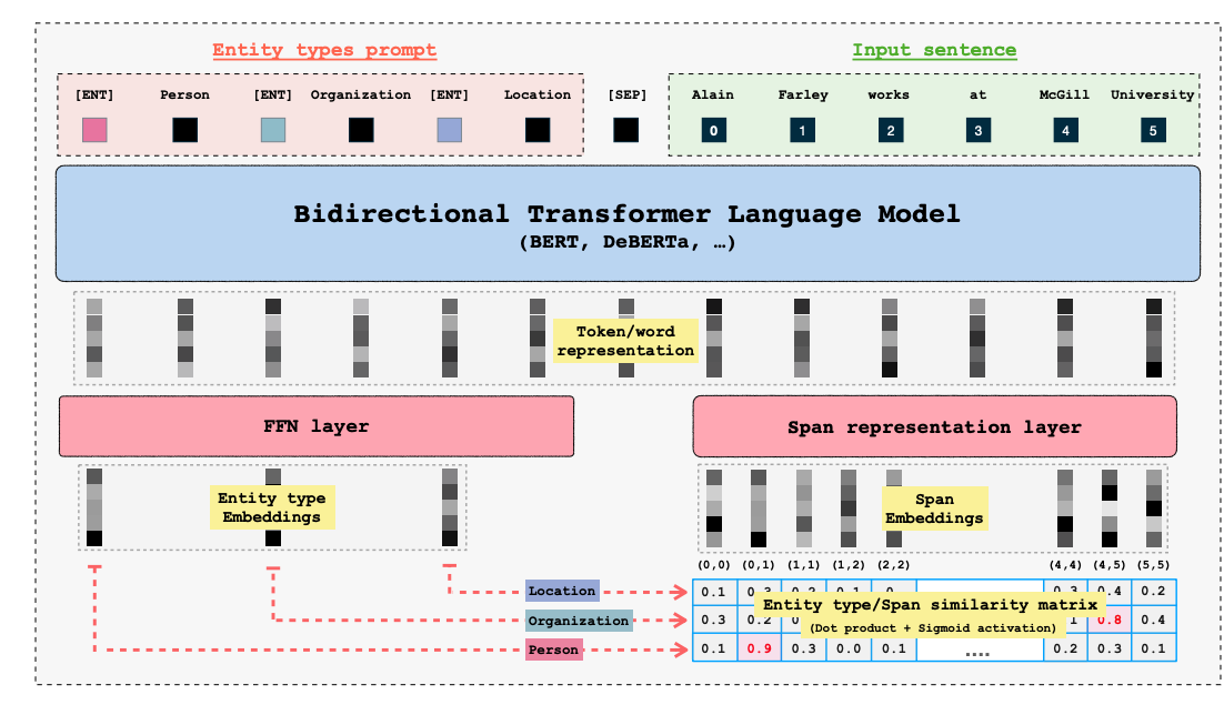
GLiNER is a compact, versatile NER model that leverages bidirectional transformers like BERT to identify a wide range of entity types overcoming the limitations of traditional models that are restricted to predefined entities. Unlike large autoregressive models, GLiNER treats NER as a task of matching entity types with spans in text, using parallel processing for efficiency. It offers a practical and resource-efficient alternative to LLMs, delivering strong performance in zero-shot scenarios without the high computational costs associated with larger models.
GLiNER architecture from the original paper<
GLiNER offers three model variants:
- GLiNER-Small-v2.1 (50M parameters)
- GLiNER-Medium-v2.1 (90M parameters)
- GLiNER-Large-v2.1 (0.3B parameters)
Compared to LLMs like Llama-3.1-70b, GLiNER models are more compact, cost-effective, and efficient for NER tasks, while LLMs generally offer broader flexibility but are much larger and resource-intensive. GLiNER medium can be tried on the Hugging Face Space: https://huggingface.co/spaces/tomaarsen/gliner_medium-v2.1 For our experiments, we focused our attention on a specific GLiNER variant EmergentMethods/gliner_medium_news-v2.1 which has been already fine-tuned on the EmergentMethods/AskNews-NER-v0 and aims at improving the accuracy across a wide range of topic and especially for long-context news entity recognition extraction.To use GLiNER you can install the gliner package based out of the Hugging Face transformers library.
!pip install gliner
Then using GLiNER for NER is as easy as:
from gliner import GLiNER

model = GLiNER.from_pretrained("EmergentMethods/gliner_large_news-v2.1")

text = """
EMCOR Group Company Awarded Contract for Installation of Process Control Systems for Orange County Water District's Water Purification Facilities
"""

labels = ["company"] # Add other entities that you want to detect here

entities = model.predict_entities(text, labels, threshold=.5)
#threshold indicates the minimum probability the model should have for the returned entities.

for entity in entities:
    print(entity["text"], "=>", entity["label"])
Output
“EMCOR Group => company"
For a list of samples the batch_text method can be used:
from gliner import GLiNER

model = GLiNER.from_pretrained("EmergentMethods/gliner_large_news-v2.1")

batch_text = [
"EMCOR Group Company Awarded Contract for Installation of Process Control Systems for Orange County Water District's Water Purification Facilities",
"Integra Eyes Orthopedics Company - Analyst Blog"
]

labels = ["company"] # Add other entities that you want to detect here

batch_entities = model.batch_predict_entities(batch_text, labels, threshold=.5)
#threshold indicates the minimum probability the model should have for the returned entities.

for entities in batch_entities:
for entity in entities:
        print(entity["text"], "=>", entity["label"])
Output:
“EMCOR Group => company" #correct predictions
"Integra Eyes Orthopedics Company => company" #incorrect predictions, ground truth Integra
The zero-shot results, in terms of F1-score on the annotated dataset of 2714 samples curated earlier is 87%.
The GLiNER model performs well in extracting company names from text but struggles with certain cases, such as when companies are mentioned as stock symbols. It also misclassifies general references to stock industries, like "Healthcare stocks" or "Industrial stocks," as company names. While effective in many cases, these errors highlight areas where further refinement is needed to improve accuracy in distinguishing between companies and broader industry terms.
- SpanMarker
SpanMarker is a framework for training powerful NER models using familiar encoders such as BERT, RoBERTa and DeBERTa. Tightly implemented on top of the 🤗 Transformers library, SpanMarker can take good advantage of it. As a result, SpanMarker will be intuitive to use for anyone familiar with Transformers. We chose this variant tomaarsen/span-marker-bert-base-orgs trained on trained on the FewNERD, CoNLL2003, and OntoNotes v5 dataset that can be used for NERn. This SpanMarker model uses bert-base-cased as the underlying encoder. It’s trained specifically to recognize organizations. It can be used for inference to predict an
ORG(organization) label as follows:
from span_marker import SpanMarkerModel

# Download from the 🤗 Hub
model = SpanMarkerModel.from_pretrained("tomaarsen/span-marker-bert-base-orgs")
# Run inference
entities = model.predict("Enernoc Acquires Energy Response; Anticipates Deal Will Add to 2013 EPS")

for entity in entities:
    print(entity["span"], "=>", entity["label"])
Output:
“EMCOR Group => ORG" #correct predictions
"Energy Response => ORG" #incorrect
The zero-shot results, in terms of F1-score on the annotated dataset of 2714 samples curated earlier is 47%. SpanMarker model performs well in extracting accurate company names but tends to identify too many incorrect entities. This is due to its training on the broader "organization" category, which includes entities such as non-profit organizations, government bodies, educational institutions, and sports teams. As a result, it sometimes confuses these with company names, leading to over-extraction and less precise results in certain contexts.
- Llama3.1-8b and Llama3.1-70b
We tested 2 variants of the Llama3.1 model including the 70b that we used to curate ground truth examples. We used the prompt that is presented above. On our annotated subset we have the following results :
| Model | Llama 3.1 8b | Llama 3.1 70b |
|---|---|---|
| F1-Score | 88% | 95% |
Performance Recap
| Model | GLiNER | SpanMarker | Llama 3.1 8b | Llama 3.1 70b |
|---|---|---|---|---|
| F1-Score | 87% | 47% | 88% | 95% |
In this experiment, we compared the performance of small models like GLiNER and SpanMarker against LLMs such as Llama 3.1-8b and Llama 3.1-70b. Small models like GLiNER (87% F1) provide a good balance between accuracy and computational efficiency, making them ideal for resource-constrained scenarios. In contrast, LLMs, while more resource-intensive, deliver higher accuracy, with Llama 3.1-70b achieving a 95% F1-score. This highlights the trade-off between performance and efficiency when choosing between small models and LLMs for NER tasks. Let’s now see how the performance differs when we fine-tune compact models.
Improving the performance of compact models with fine-tuning on LLM-assisted labeled dataset
Fine-tuning
Using our train/validation/test subsets created earlier, we fine-tuned GLiNER and SpanMarker on an AWS instance with a single Nvidia A10 GPU. A fine-tuning example for GLiNER is accessible here and for SpanMarker here. Fine-tuning those models is as easy as running this with train_datasetand valid_datasetcreated as Hugging Face dataset.
import numpy as np
from gliner import GLiNER, Trainer
# calculate number of epochs
batch_size = 4
learning_rate=5e-6
num_epochs = 20
model=GLiNER.from_pretrained("EmergentMethods/gliner_medium_news-v2.1")
    data_collator = DataCollator(model.config, data_processor=model.data_processor, prepare_labels=True)
    log_dir = create_log_dir(model_path, model_name, learning_rate, batch_size, size, model_size, timestamp=False)
    training_args = TrainingArguments(
        output_dir=log_dir,    # Optimizer, model, tokenizer states
        logging_dir = log_dir,
        overwrite_output_dir = 'True',
        learning_rate=learning_rate,              	# Learning rate
        weight_decay=0.01,                        	# Weight decay
        others_lr=1e-5, 					     # learning rate
        others_weight_decay=0.01,                 	# weight decay
        lr_scheduler_type="linear",        # learning rate scheduler
        warmup_ratio=0.1,                  # Warmup steps ratio
        per_device_train_batch_size=batch_size,   	# Training batch
        per_device_eval_batch_size=batch_size,    # Evaluation batch
        focal_loss_alpha=0.75,          # Focal loss alpha parameter
        focal_loss_gamma=2,             # Focal loss gamma parameter
        num_train_epochs=num_epochs,              # training epochs
        save_strategy="epoch",          # Save the model at the end of each epoch
        save_total_limit=2,             # Keep only the best model
        metric_for_best_model="valid_f1",
        use_cpu=False,                  # Use GPU
        report_to="tensorboard",        # Report to TensorBoard
        logging_steps=100,              # Steps between logging
        evaluation_strategy="epoch",    # Evaluate every few steps
    )

trainer = Trainer(
    model=model,
    args=training_args,
    train_dataset=train_dataset,
    eval_dataset=valid_dataset,
    tokenizer=model.data_processor.transformer_tokenizer,
     data_collator=data_collator,
     compute_metrics=custom_compute_metrics
     )
    trainer.train()
The training ran for 20 epochs, we save the checkpoint with the highest F1 score on the validation set.
Performance comparison
| Model | gliner-medium-news | Gliner-medium-news finetuned | SpanMarker | SpanMarker fine-tuned | Llama 3.1 8b | Llama 3.1 70b |
|---|---|---|---|---|---|---|
| Test set F1-Score | 87.0% | 93.4% | 47.0% | 90.1% | 80.0% | 92.7% |
In this updated comparison, we evaluated models based on their F1-scores after fine-tuning. The GLiNER-medium-news model improved from 87.0% to 93.4% after fine-tuning, showing significant gains in accuracy. Similarly, SpanMarker went from 47.0% to 90.1% with fine-tuning, making it far more competitive. Meanwhile, Llama 3.1-8b and Llama 3.1-70b performed well out of the box, scoring 80.0% and 92.7%, respectively, without fine-tuning. This comparison emphasizes that fine-tuning smaller models like GLiNER and SpanMarker can dramatically enhance performance, rivaling larger LLMs at a lower computational cost.
The llama 3.1-70b model costs at least $8 per hour for inference, making it significantly more expensive than compact models, which can run on a GPU instance costing around $0.50 per hour—16 times cheaper. Furthermore, compact models can even be deployed on CPU instances, costing as little as ~$0.10 per hour, which is 80 times less expensive. This highlights the substantial cost advantage of smaller models, especially in resource-constrained environments, without sacrificing competitive performance when fine-tuned for specific tasks.
Weak Supervision vs. LLM-assisted labeling
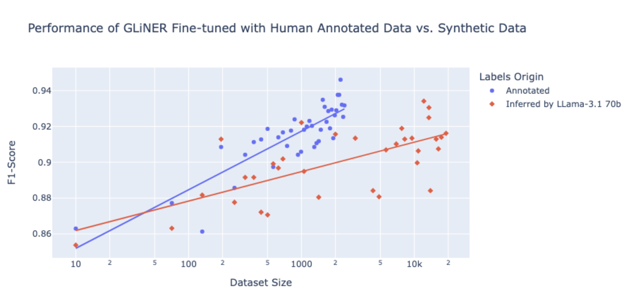
In this experiment, we explored two key approaches to data labeling for NER: Weak Supervision and LLM-assisted labeling. While weak supervision enables scalable training on synthetic data, our findings suggest that it cannot achieve the same level of accuracy as models trained on manually annotated data. For 1,000 samples, manual annotation took 3 hours with an F1 score of 0.915, while Llama 3.1-70b inference only took 2 minutes but resulted in a slightly lower F1 score of 0.895. The trade-off between speed and accuracy depends on the task's requirements.
Weak Supervision vs. LLM-assisted labeling
The graph compares the performance of GLiNER fine-tuned on human-annotated data versus synthetic data inferred by Llama-3.1 70b across varying dataset sizes. The blue dots represent F1-scores of models trained on human-annotated data, while the red dots represent those inferred by Llama-3.1 70b. As dataset size increases, models fine-tuned on human annotations consistently outperform those using synthetic data, achieving higher F1-scores. It illustrates that while models fine-tuned on human annotations yield higher accuracy,_ LLM-assisted labeling using Llama-3.1 70b can still provide considerable value, especially when resources for manual annotation are limited. Even though the F1-scores from LLM-inferred data are slightly lower, they remain competitive across various dataset sizes. LLMs can rapidly generate large volumes of annotations, offering a practical solution for scaling dataset creation efficiently, making them beneficial in scenarios where time and cost constraints are critical.
Conclusion
Our experiment demonstrated that while large models like Llama 3.1 provide superior performance out of the box, fine-tuning smaller models like GLiNER and SpanMarker with LLM-assisted labeling can significantly enhance accuracy, rivaling the LLMs at a fraction of the cost. This approach highlights how investing in fine-tuning small models using LLM insights provides a cost-effective, scalable solution for financial NER tasks, making it ideal for real-world applications where both accuracy and resource efficiency are crucial.
